Probability and Statistical Inference

Summary of lectures

Lecture 1 - 19/09/2018

Introduction & Fundamentals

Introduction

(comic strips):
- Data Analysys:
  - The gathering, display, and and summary of data.
- Probability:
  - The laws of chances, in and out of the casino.
- Statistica Inference
  - The science of Drawing statistical conclusions from specific data, using a knownkedge of probability.
What is the module about:
- For the purposes of a Statistical Inquiry
  - How to collect and prepare data for use
  - How to describe the data (in terms of format and statistically)
  - How to formulate, state, test and report on hypotheses
  - How to conduct exploratory and predictive analytics
  - How to use an appropriate software package
    - We will be using R
  - How to report your findings correctly
How to succeed in the module
- Focus on learning the process of conducting a statistical analysis
  - What are you trying to discover or show?
    - Figure out a question you are trying to answer/theory you are trying to test
  - What data do you need to collect?
  - Once you have data, how do you describe the data you have?
    - You need to explain this to whoever will be the consumer of your work
  - What analysis should you conduct?
    - You need to know the types of tests to run and how to explain this to your consumer
  - How do you interpret your analysis?
    - You need to know how to interpret the outcomes of the analysis and present these to your consumer
  - How will you present your findings?
  - Present the question you are interested in
    - In a way that makes sense to conduct a statistical analysis
  - Inspect and prepare the data you have
    - To support a statistical analysis
  - Describe the data you have
    - In a way that your consumer can understand any constraints the data may put on your analysis
  - Conduct a statistical analysis
    - Using appropriate statistical tests
  - Report on your statistical analysis
    - In a way that makes sense for your consumer
  - Interpret the outcomes of your statistical analysis
    - Drawing appropriate conclusions
  - Report on the findings of your statistical analysis
    - In a way that makes sense for your consumer

Fundamentals

Types of Data Analysis
- Qualitative Methods
  - Testing theories using language
- Quantitative Methods
  - Testing theories using numbers (via statistics)
- statistical inquiry:
  - science of collecting, analysing, and drawing conclusions from data
  - science of collecting, describing, and interpreting data.
  - objectively and quantitatively
  - Is usually carried out with a SAMPLE
The Research Process (Andy Field)
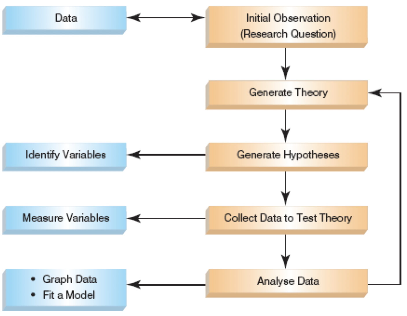
- Inital Observation (Research Question)
  - Data
    - Find something that needs explaining
    - Read other research
    - Test the concept
      - collect data that will provide evidence you can test to see if your idea is valid
    - Define variables that can be measured and can differ across entities or time
- Generate Theory
  - Theory: A hypothesized general principle or set of principles that explains known findings about a topic and from which new hypotheses can be generated. e.g. Computer Science attracts students with strong mathematical ability.
- Generate Hypotheses
  - Identify Variables.
    - Hypotheses: A prediction from a theory. E.g. the number of people applying for an MSc in Computer Science will have basic mathematical ability greater than the general level in the population.
    - Falsification: The act of disproving a theory or hypothesis.
- Collect Data to Test Theory
  - Measure Variables
    - What data am I interested in/do I need?
      - Population: The entire set of individuals or objects of interest or the measurements obtained from all individuals or objects of interest
        
        finite or infinite.
      - Sample: A portion, or part, of the population of interest
        
        Statistical inquiry is usually carried out with a SAMPLE
        
        If Sample is not representative it is biased.
        
        Factors influencing the accuracy of a sample’s ability to represent a population: size and randomness.
      - Individuals: people or objects being studied
        
        The set of data of an individua is referred to as a case.
      - Variable: A characteristic about each individual.
        
        Any characteristic whose value may change from one individual to another.
      - Data: Value of a variable for individual observations.
      - Dataset: The set of values collected for the variable(s) from each of the individuals belonging to the sample/population the dataset represents.
        
        Each case in a dataset has one datum or observation for each variable.
      - Experiment: A planned activity whose results yield a set of data.
      - Parameter: A numerical value describing an aspect of an entire population.
        
        For small populations it is possible to measure to compute a parameter
      - Statistic: A numerical value describing an aspect of the sample.
        
        For larger populations you will measure to compute a statistic
  - Example:
```
  A country is interested in learning about the average age of its academic staff working at third level.
  The basic terms in this situation:

  - The population is all academic members working in the country and we want to determine their age.
  - A sample is any subset of that population.  
      - For example, we might select 50 staff members and determine their age.
      As long as this is representative and sufficiently large to model the population.
  - The variable is the “age” of each staff member.
  - One datum would be the age of a specific faculty member.
  - The experiment would be the method used to select the ages forming the sample and determining the actual age of each staff member in the sample.
  - The parameter of interest is the “average” age of all academic staff in the country.
  - The statistic is the “average” age for all academic staff in the sample.
```
  - Biased Sampling Method:
    - A sampling method that produces data which systematically differs from the population from which it is taken.
  - Aim for a Simple Random Sample
    - A sample of n measurements from a population is a subset of the population selected in such a manner that every sample of size n from the population has an equal chance of being selected
  - Data Collection: What to Measure? Eg.:
```
  Hypothesis: Consumption of Coca-Cola improves a student’s ability to concentrate.
  Decide what variables you need.
  Independent Variable:
      - The proposed cause
      - Predictor variable
      - Manipulated variable (in experiments)
      - Coca-Cola consumption in the hypothesis above
  Dependent Variable:
      - The proposed effect
      - An outcome variable
      - Measured not manipulated (in experiments)
      - A student’s ability to concentrate in the hypothesis above
```
  - Qualitative, or Attribute, or Categorical, Variable
    - A variable that categorizes or describes an element of a population.
    - Identifies basic differentiating characteristics of the population.
      
      Note: Arithmetic operations, such as addition and averaging, are not meaningful for data resulting from a qualitative variable.
  - Quantitative, or Numerical, Variable
    - A variable that quantifies an element of a population.
    - Observations or measurements take on numerical values
      
      Note: Arithmetic operations such as addition and averaging, are meaningful for data resulting from a quantitative variable.
    - Discrete:
      - Isolated points along a number line
      - Usually counted
      - Can only take certain values
      - E.g. rolling a dice, #students attending class
    - Continuous
      - Variable that can be any value in a given range
      - Usually measured
      - E.g. heights of students attending class, time spent concentrating in class
  - Levels of measurement
    - Nominal
      - Data can be assigned to a category
    - Ordinal
      - There is a ranking associated with the variable
      - Data can be ordered from smallest to largest, best to worst etc.
    - Interval
      - Data can be ordered but there is meaning between the values of order
      - Allows comparison between the data values Ratio
      - Data can be ordered, there are differences between the values and you can find the ratio
      - Has an absolute 0
      - It makes sense to say for example one value is twice as large as another
      - Interval and Ration may be referred to as Scale
- Analyse Data
  - Graph Data
  - Fit a Model
  - Summarizing vs Analysing:
    - Descriptive Statistics
      - Describing the population and the sample
      - Summarizing
    - Inferential Statistics
      - Inference from sample to population
      - Inference from statistic to parameter
    - Using the appropriate statistical tests to draw inference
Measure of Central Tendency
- A single number to serve as a representative value around which all the numbers in the set tend to cluster.
Mode: The value with the greatest frequency on the distribution.
- The mode is not a very useful measure of central tendency
- Two data sets that are very different from each other can have the same mode
- The mode is primarily used with nominal variables
- Eg.:
  - 3, 7, 5, 13, 20, 23, 39, 23, 40, 23, 14, 12, 56, 23, 29
  - In order these numbers are:
  - 3, 5, 7, 12, 13, 14, 20, 23, 23, 23, 23, 29, 39, 40, 56
  - In this case the mode is 23.
- Bimodal Distributions:
  - When a distribution has two “modes,” it is called bimodal
- Multimodal Distributions
  - If a distribution has more than 2 “modes,” it is called multimodal
Median
- It is the score in the middle
- The middle score of a sequence of all the scores in a distribution arranged from lowest to highest.
- Eg.:
  - Sort the data from highest to lowest
  - Find the score in the middle
    - middle = (N + 1) / 2
    - If N, the number of scores, is even the median is the average of the middle two scores eg.:
    - 10 8 14 15 7 3 3 8 12 10 9
    - Sort the scores:
    - 15 14 12 10 10 9 8 8 7 3 3
    - Determine the middle score:
    - middle = (N + 1) / 2 = (11 + 1) / 2 = 6
    - Middle score = median = 9 eg2:
    - 24 18 19 42 16 12
    - 42 24 19 18 16 12
    - middle = (N + 1) / 2 = (6 + 1) / 2 = 3.5
    - Median = average of 3rd and 4th scores:
    - (19 + 18) / 2 = 18.5
The Mean
- The arithmetic average of a group of scores
- Summing up all the observation and dividing by number of observations.
- eg.:
  - 1 5 4 3 2
  - 1 + 5 + 4 + 3 + 2 = 15
  - 15 / 5 = 3
- The mean is sensitive to extreme values
Measures of Dispersion
- Descriptive statistics that describe how similar a set of scores are to each other (or the range of scores)
  - The more similar the scores are to each other, the lower the measure of dispersion will be
  - The less similar the scores are to each other, the higher the measure of dispersion will be
  - In general, the more spread out a distribution is, the larger the measure of dispersion will be
  - 3 main measures:
    - The range
      - difference between the largest and smallest score in the set of data:
        
        4 8 1 6 6 2 9 3 6 9
        
        XL=9; XS=1
        
        Range = XL - XS = 8
      - is used when mainly for ordinal data
      - rarely used in scientific work
      - Two very different sets of data can have the same range
    - Variance / standard deviation
      - Variance:
        
        Concerned with deviations from the mean (X-µ)
        
        It’s the average of the squared differences from the mean
        
        First subtract the mean from each of the scores
        
        This difference is called a deviate or a deviation score
        
        The deviate tells us how far a given score is from the typical, or average, score
        
        Thus, the deviate is a measure of dispersion for a given score
        
        Then square the result
        
        Because if we just added up the differences from the mean the negatives would cancel the positives
        
        Also, If we used absolute values we wouldn’t get an accurate measure of spread
        
        Variance is defined as the average of the deviations from the mean squared:
        
        N here is the degrees of freedom (DF):
        
        the number of independent pieces of information on which the estimate is based
      - standard deviation
        
        Standard deviation = the square root of the Variance
        
        The standard deviation is the most useful and the most popular measure of dispersion.
        
        ** Used to calc margens of the mean. Eg: group is from (mean - SD) until (mean + SD)
        
        Also helpful in comparing samples.
        
        Greek symbol sigma σ
        
        The larger the value the more spread out around the mean the data is, smaller means less spread.
        
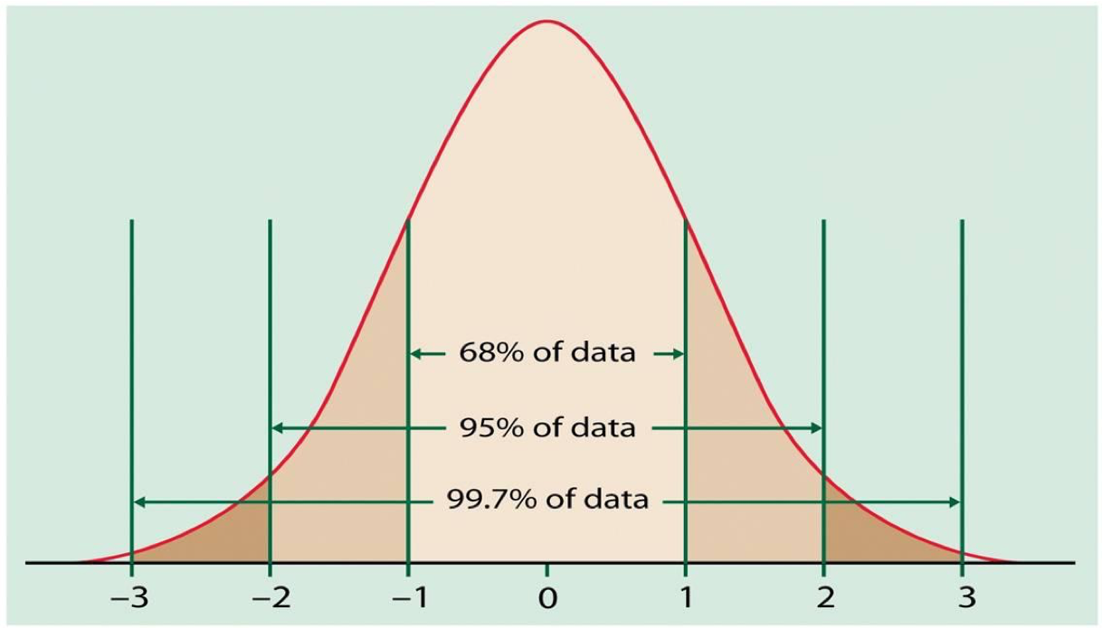
        The 68-95-99.7 Empirical Rule In the normal distribution with mean µ and standard deviation σ:
        
        68% of the observations fall within σ of the mean µ.
        
        95% of the observations fall within 2σ of the mean µ.
        
        99.7% of the observations fall within 3σ of the mean µ.
        
        ** Eg.: If you compare 2 Data Sets with the same mean score for Probability and Statistics, it doesn’t mean they will have the same performance, as SD may be diff.
    - The Interquartile Range (IQR)
      - the difference of the first (25th percentile) and third (75th percentile) quartiles divided by two
      - IQR = (Q3 - Q1) / 2
      - Eg: IQR of 2, 4, 6, 8, 10, 12, 14, 20, 30, 60:
        
        (25 - 5) / 2 = 10
Measure of Skew
- Skew is a measure of symmetry in the distribution of scores
- Normal distributions: mean = median = mode
- Positively skewed distributions: mean > median
- Negatively skewed distributions: mean < median
Kurtosis
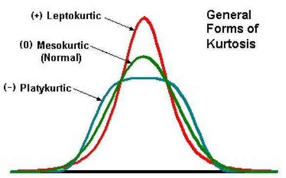
- measures whether the scores are spread out more or less than they would be in a normal (Gaussian) distribution
- Distribution Normal == 3 == mesokurtic
- Distribution less spread == kurtosis > 3 == leptokurtic
- Distribution more spread == kurtosis < 3 == platykurtic
Mean or Median
- The median is less sensitive to outliers (extreme scores) than the mean and thus a better measure than the mean for highly skewed distributions, e.g. family income.
- Median is more reflective of the data.
- Eg:
  - Mean of 20, 30, 40, and 990 is (20+30+40+990)/4 =270.
  - Median of these four observations is (30+40)/2 =35.
  - 3 observations out of 4 lie between 20-40.
  - Mean of 270 really fails to give a realistic picture of the major part of the data.
When to use Median & IQR:
- The median is often used when the distribution of scores is either positively or negatively skewed
  - The few really large scores (positively skewed) or really small scores (negatively skewed) will not overly influence the median
- The IQR is often used with skewed data as it is insensitive to the extreme scores
Mean and Standard Deviation
- You should use the mean when
  - the data are interval or ratio scaled
    - Many people will use the mean with ordinally scaled data too
  - and the data are not skewed
- The mean is preferred because it is sensitive to every score
- If you change one score in the data set, the mean will change
- If you use mean you also use standard deviation
Key concepts:
- Sample: Size, representativeness, extremes Differing types of variable: nominal/categorical, ordinal, interval and ratio Measures of central tendency: the mean, median and mode Measures of dispersion: range, inter-quartile range, variance and standard deviation Shape: normal, skew, kurtosis

Lecture 2 - 19/09/2018

Describing and Presenting Data

Source of the class:
- Statistics and Data Analysis, Peck, Olsen and Devore
- Discovering Statistics Using IBM SPSS (equivalent R book), Andy Field
- Understanding Basic Statistics, Brase and Brase
Webcourses portal: Download content (Week 2):

File geoms.docx (843.268 KB)
File PSIWeek2.R (6.032 KB)
File L2-More on Describing Data.pptx (2.435 MB)
File PSIWeek2Data.zip (12.167 KB)
File Datasets.docx (14.26 KB)

Attached to this page you will find the material you need for the lecture tomorrow plus the practical class.

geoms.docx is a scan of pages from Andy Field's book about common geom functions and aethetics
Datasets.docx describes the data we are using.
PSIWeek2Data.zip contains the datasets we are going to use.
PSIWeek2.R includes the R script for creating some graphs from the lecture.

Statistics: Science of collection, presentation, analysis, and reasonable interpretation of data.
- Statistics provides a rigorous scientific method for gaining insight into data.
Experiements and variables:
- Variable: Things we can manipulate, Compute, Or control for
- X is a variable, x is the value of the variable
- Random variable
  - is determined by chance
- Discrete random variable
  - May only take on a finite number of values or countable number of values
  - Result of a count
- Continuous random variable
  - May take on any number of values in a line interval
  - Measured on a continuous scale
Describe for numerical data
- Centre: Discuss where the middle of the data falls
  - Measures of central tendency
  - mean, median and mode
- Spread: Discuss how spread out the data is
  - Refers to the variability in the data
  - Range, standard deviation, IQR
- Shape: Refers to the overall shape of the distribution
  - Symmetrical, uniform, skewed, or bimodal
- Unusual Occurrences like Outliers (value that lies away from the rest of the data), Gaps and Clusters
- Contextualize using correct statistical vocabulary and complete sentences.
Trimmed mean: remove outliers from a data set
- Use case eg.:
  - Example Olympic Diving/Gymnastics scoring: eliminate extreme scores/bias from judges.
- Not often used for large datasets
- Calculate as per:
  1. Multiply the percent to trim by n (number in the sample)
  2. Truncate that many observations from BOTH ends of the distribution (when listed in order)
  3. Calculate the mean with the shortened data set
    - Eg.: 12, 14, 19, 20, 22, 24, 25, 26, 26, 50
    - Mean: 23.8
    - 10% trimmed = 10%(10) = 1
    - Removed trimmed observation (1) of each side: 12, 14, 19, 20, 22, 24, 25, 26, 26, 50
    - Trimmed mean = (14, 19, 20, 22, 24, 25, 26, 26)/8 = 22
Methods of Variability/Dispersion Measurement
- Commonly used: Range, variance, standard deviation, interquartile range, coefficient of variation etc.
- 3 data sets can have the samen mean and meddian, but different amounts of variability.
Types of Variation:
- Systematic Variation
  - Differences in performance created by a specific experimental manipulation.
- Unsystematic Variation
  - Differences in performance created by unknown factors.
  - Age, gender, IQ, time of day, measurement error, etc.
- Randomization
  - Minimizes unsystematic variation.
Degrees of freedom
- - DF = number of items - 1
- Is the number of independent pieces of information that went into calculating the estimate.
- Another way to look at degrees of freedom is that they are the number of values that are free to vary in a data set.
- Or the number of values that need to be known in order to know all the values needed to achieve a particular value.
- If you have two samples and want to find a parameter, like the mean, you have two “N”s to consider (sample 1(N1) and sample 2(N2)).
  - DF in that case is: (N1 + N2) – 2.
Measures of Variability:
- Interquartile range advantage over the standard deviation:
  - IQR is resistant to extreme values
- Interquartile range (IQR) is the range of the middle half of the data.
- Lower quartile (Q1) is the median of the lower half of the data
- Upper quartile (Q3) is the median of the upper half of the data
Which Descriptive Statistic to use? (Key slide)
- Depends on measurement type and data dispersion
- Interval or Ratio (Scale)
  - Normally distributed
    - Mean and Standard Deviation
  - Skewed
    - Median and Interquartile Range
  - Ordinal or nominal
    - Mode and/or simple frequencies
Analysing Data
- First step: Graph the data
- Frequency Distributions (aka Histograms)
- Ideal: The ‘Normal’ Distribution (Bell-shaped, Symmetrical around the centre)
Properties of Frequency Distributions: Skew, Kurtosis
Probability: Chance behaviour is unpredictable in the short term, but has a regular and predictable pattern in the long term.
Sample Space: The set of all possible outcomes of a random phenomenon
Event: Any set of outcomes of interest
Probability of an event: The relative frequency of this set of outcomes over an infinite number of trials
P(A) is the probability of event A
- P(X = 1) refers to the probability that the random variable X is equal to 1.
- P(X<=x) is a Cumulative probability. The probability that a value falls within a particular range or interval
Discrete Random Variable
- The sum of all assigned probabilities must be 1
- Mean is often called the expected value
  - Represents a cluster point for the entire distribution
- Standard deviation is represented as a measure of risk
  - Larger the standard deviation, the more likely it is that a random variable x is different from the expected value
Discrete Probability Distribution
- Shows us the complete space on which the distribution is based
- The corresponding probability of each event in the sample space

Probability Distributions

Flipping a coin twice. Possible outcomes: HH, HT, TH, and TT.
- If X is number of Heads resulted, thus X can take on the values 0, 1, or 2.
- X is a random variable because its value is determined by the outcome of a statistical experiment.
is a table or an equation that links each outcome of a statistical experiment with its probability of occurrence.

Number of heads(X)	Probability
0	0.25
1	0.50
2	0.25

Probability of X=the number of Heads that result from this experiment
A cumulative probability refers to the probability that the value of a random variable falls within a specified range.
If we flip a coin two times, what is the probability that the coin flips would result in one or fewer heads? Cumulative probability:
- P(X < 1) = P(X = 0) + P(X = 1) = 0.25 + 0.50 = 0.75

Number of heads(X)	Probability: P(X = x)	Cumulative Probability: P(X < x)
0	0.25	0.25
1	0.50	0.75
2	0.25	1.0

The simplest probability distribution occurs when all of the values of a random variable occur with equal probability.
Suppose the random variable X can assume k different values.
Therefore, If P(X=x_k) is constant, then, P(X=x_k)=1/k
What is the probability that the die will land on 5?
- Possibilities: S = { 1, 2, 3, 4, 5, 6 }
- Thus, we have a uniform distribution. Therefore, the P(X=5)=1/6.
what is the probability that the die will land on a number that is smaller than 5?
- Cumulative probability:
 - P( X < 5 ) = P(X = 1) + P(X = 2) + P(X = 3) + P(X = 4) = 1/6 + 1/6 + 1/6 + 1/6 = 2/3
Continuous Probability Distribution: When a random variable is a continuous variable (variable can take on any value between two specified values).
cannot be expressed in tabular form
- An equation or formula (probability density function) is used
Hypothesis testing relies extensively on the idea that, having such a function, one can compute the probability of all the corresponding events i.e.
- probability of a X taking a value less than or equal to a particular value (a)

Calculating Probability from a Frequency distribution

Statisticians have created a range of idealized distributions probability distributions and from these we can calculate the likelihood of achieving particular values if our data distribution matches.

If we have data shaped like the normal distribution then the mean can be mapped to 0 and the standard deviation to 1
We can then use the tables of probability created by these statisticians to work out the probability of particular scores occurring within that distribution

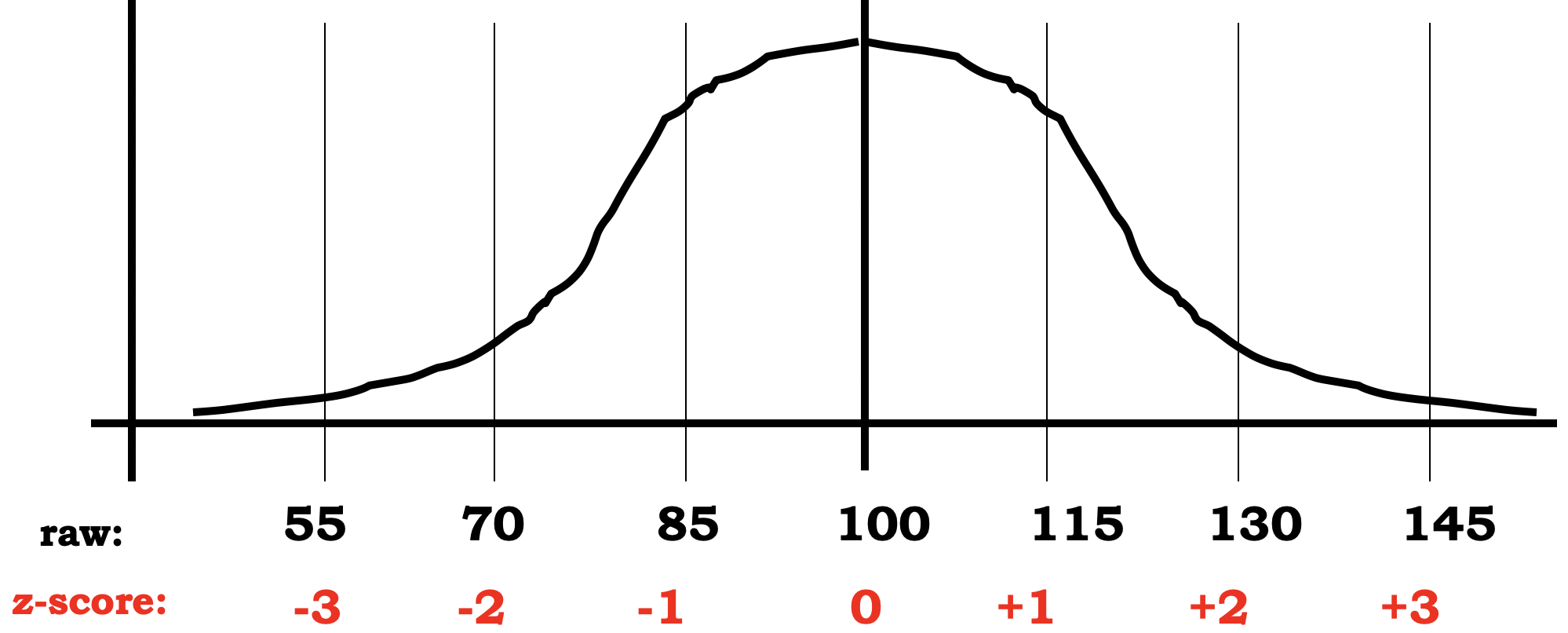
z-scores has a mean of 0 and SD = 1

Z score states the position of a raw score in relation to the mean of the distribution, using the standard deviation as the unit of measurement.
- Z = (Raw score - mean) / SD
For population:
- Z = (X - μ) / σ
For sample:
- Z = (X - x̅) / s
z-scores transform our original IQ scores into scores with a mean of 0 and an SD of 1.
Raw IQ scores (mean = 100, SD = 15)
z for 100 = (100-100) / 15 = 0, z for 115 = (115-100) / 15 = 1,
z for 70 = (70-100) / -2, etc.
The probability that a realization is lower than point 2.33 = 0.99
- (See on internet Table of the Normal Distribution)

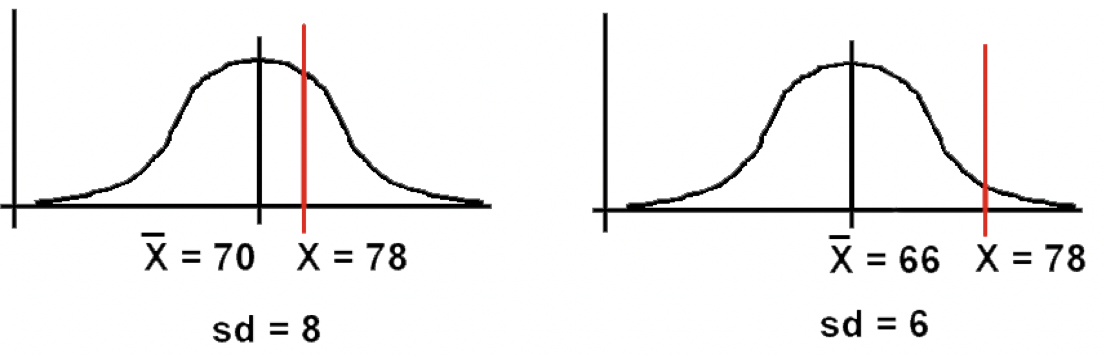
Use case of z-score:

Test A: Fred scores 78. Mean score = 70, SD = 8.
Test B: Fred scores 78. Mean score = 66, SD = 6.
Did Fred do better or worse in comparison to the rest of the class on the second test?
Test A: as a z-score, z = (78-70) / 8 = 1.00
Test B: as a z-score , z = (78 - 66) / 6 = 2.00
Conclusion: Fred comparatively did much better on Test B.
z-scores enable us to determine the relationship between one score and the rest of the scores, using just one table for all normal distributions.

Eg 2: If we have 480 scores, normally distributed with a mean of 60 and an SD of 8, how many would be 76 or above? Z-Score Example 2

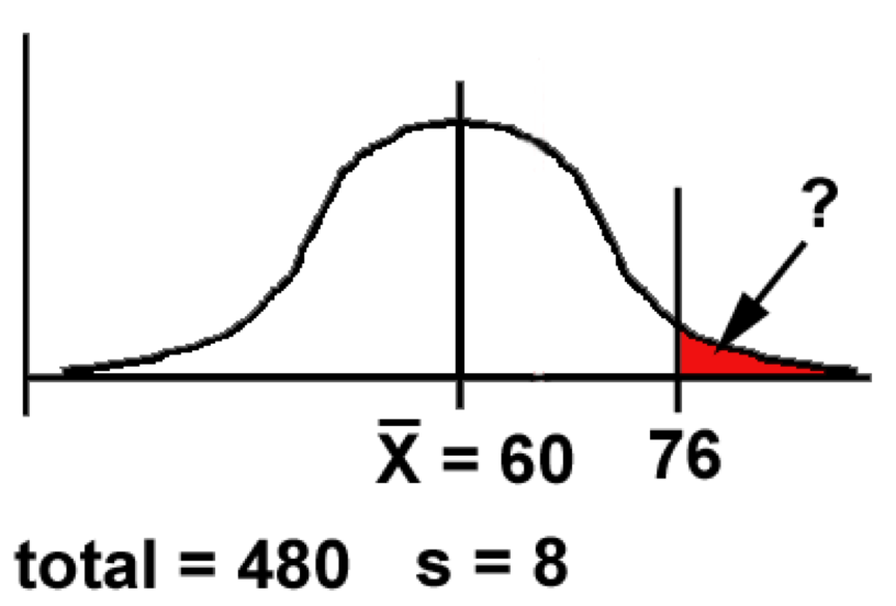
Work out the z-score for 76:
z = (X - x̅) / s = (76 - 60) / 8 = 16 / 8 = 2.00
We need to know the size of the area beyond z.
Looking at the table, we find

Z	(a) Area btw Mean and Z	(b) Area beyond Z
2.00	0.4772	0.0228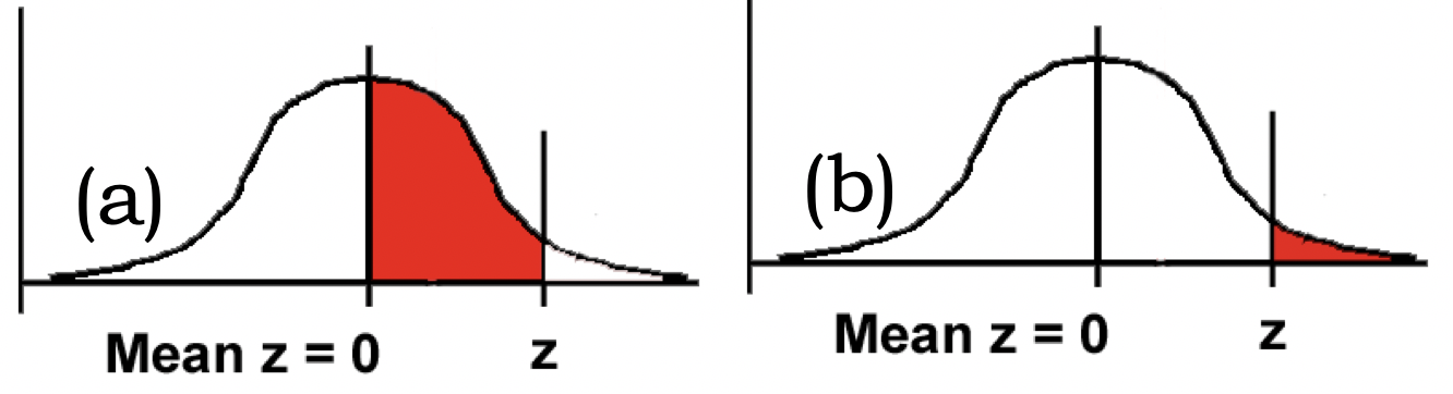

Z-Score Example Table

So: as a proportion of 1, 0.0228 of scores are likely to be 76 or more.
As a percentage, = 2.28%
As a number, 0.0228 * 480 = 10.94 scores.

Eg 3: Word comprehension test scores:
- Person with no brain damage: no. correct: mean = 92, SD = 6 out of 100
- Brain-damaged person: no. correct: 89 out of 100.
- Is this person’s comprehension significantly impaired?
- Step 1: Graph the problem:
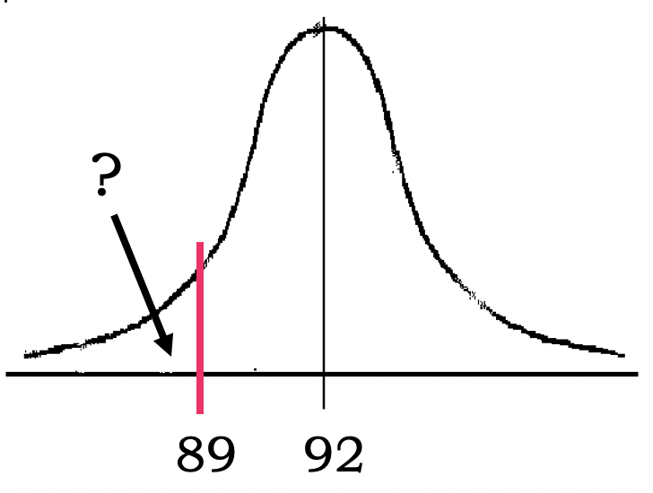
- Step 2: Convert 89 into a z-score:
  - z = (89 - 92)/6 = - 3/6 = -0.5
- Step 3: use the table to find the “area beyond z” for our z of - 0.5:
  - Area beyond z = 0.3085
- Conclusion: .31 (31%) of people without brain damage are likely to have a comprehension score this low or lower.

The Normal Distribution
- Normal Curve, Bell-shaped Curve or Gaussian distribution
- It’s symmetrical around the mean.
- The mean, median and mode all have same value.
- It can be specified completely, once mean and SD are known.
- The area under the curve is directly proportional to the relative frequency of observations.
  - Thus we can calculate the probability of observations occurring in a population The Empirical Rule
- 68% of the observations fall within σ of the mean µ.
- 95% of the observations fall within 2σ of the mean µ.
- 99.7% of the observations fall within 3σ of the mean µ.
- Z-Score properties:
  - 1.96 cuts off the top 2.5% of the distribution.
  - −1.96 cuts off the bottom 2.5% of the distribution.
  - As such, 95% of z-scores lie between −1.96 and 1.96.
  - 99% of z-scores lie between −2.58 and 2.58,
  - 99.9% of them lie between −3.29 and 3.29.
Distribution is central to choosing the correct test
- Parametric Tests
  - Normal distribution
- Non-parametric Tests
  - Non normal distribution
- Always start by looking at the data!
Population
- The collection of units (be they people, plankton, plants, cities, suicidal authors, etc.) to which we want to generalize a set of findings or a statistical model
Sample
- A smaller (but hopefully representative) collection of units from a population used to determine truths about that population
outcome_i=(model)+error_i
- In statistics we fit models to our data
- The mean is a hypothetical value
  - As such, the mean is simple statistical model.
- How can we assess how well the mean represents reality?
  - Calculating ‘Error’:
    - deviation = x_i - x̅ Total Error: (sum the deviations)
      - Σ(x_i - x̅)
      - We could add the deviations to find out the total error.
      - Deviations cancel out because some are positive and others negative.
      - Therefore, we square each deviation.
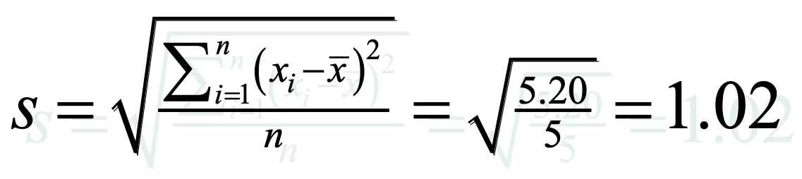
      - SS=Σ(x_i - x̅)²
  - Variance:
    - The sum of squares is a good measure of overall variability, but is dependent on the number of scores.
    - We calculate the average variability by dividing by the number of scores (n).
    - This value is called the variance (s2).
    - variance(s²) = SS/N-1 = Σ(x_i - x̅)²/N-1
    - The variance has one problem: it is measured in units squared.
    - This isn’t a very meaningful metric so we take the square root value (measured in units).
    - This is the standard deviation (s).
  - Standard Deviation
Important to remember:
- The sum of squares, variance, and standard deviation represent the same thing:
- The ‘fit’ of the mean to the data
- The variability in the data
- How well the mean represents the observed data
- Error
Standard error of the mean (SE)
- **When you calculate the Standard Deviation of sample means
  - means of many samples of the same Population, in order to estimate the mean of the entire population
- Central Limit Theorem
  - As samples get large, the sampling distribution has a normal distribution with a sample mean equal to the population mean and a standard deviation of
    - σ_x̅=S / √N̅
  - We can use the standard deviation of the sampling distribution as the approximation of the sample error
    - If our distribution follows the normal distribution
Confidence Intervals (CI)
- CI represents a range of values between which we think a population value will fall
- Compute the mean of a sample in order to estimate the mean of the population.
  - Clearly, if you already know the population mean, there would be no need for a Confidence Interval.
- Eg.: Suppose we are looking at our fish in Lough Mask
  - True mean: 15 thousand fish
  - Sample mean: 17 thousand fish
  - Interval estimate:
    - 12 to 22 thousand(contains true value)
    - 16 to 18 thousand (misses true value)
    - CIs constructed such that 95% contain the true value.
- Typically look at 95% CI but can also look at 99%
- What does this mean?
  - If we say CI is 95% then if we collected 100 samples, calculated the mean
  - Then a CI of 95% means we are confident that 95 of these would contain the true mean
- How to calculate?
  - Need to know the limits within which 95% of the means fall
  - Go back to the normal distribution – 95% of scores fall between +-1.96
  - Once we know the mean and standard deviation we can calculate any score and therefore the CI
    - Lower boundary: X̅=1−SE
    - Upper boundary: X̅= 1+SE
      - X̅ = population mean, SE = standard error of the mean
Graphical presentation: (Key slide)
- Nominal or Ordinal:
  - Bar charts, Pie charts or Frequency Tables
- Interval or Ratio numerical:
  - Histogram, Stem and Leaf diagrams or Box-plot
    - Depending on dispersion
- Stem-and-Leaf plot
  - Shows data arranged by place value.
  - You can use a stem-and-leaf plot when you want to display data in an organized way that allows you to see each value.
    - Use for small to moderate sized data sets.
  - Accompany with a comment on the centre, spread, and shape of the distribution and if there are any unusual features.
- Histogram
  - Use for univariate numerical data (one variable)
  - To compare two or more histograms, use the same scale on the horizontal axis
  - Describe it as per example:
  - “The median number of hours spent watching TV per day was greater for the 1-year-olds than for the 3-year-olds. The distribution for the 3-year-olds was more strongly skewed right than the distribution for the 1-year-olds, but the two distributions had similar ranges.”

Lecture 3 - 19/09/2018

Correlation and Difference

Sources of the class:
- Statistics and Data Analysis, Peck, Olsen and Devore
- Discovering Statistics Using IBM SPSS (And equivalent R book), Andy Field
- Understanding Basic Statistics, Brase and Brase
- SPSS Survival Manual, Julie Pallant
Webcourses portal: Download content (Week 3):

File PSIWeek3-Lecture.Rmd (6.118 KB)
File Field-BDI-Non-parametric.dat (466 B)
File L3 - Correlation and Difference.pptx (3.075 MB)
File PSIWeek3-Lecture.html (958.808 KB)
File PSIWeek3Exercise.docx (198.319 KB)
File survey.dat (192.817 KB)
File Regression.sav (190.589 KB)
This week we are introducing statistical tests for correlation and difference.

Attached to this page you will find:

Lecture notes (.pptx)
PSI-Week3.rmd - R markdown file with all the commands used in the lecture + PSIWeek3-Lecture.html which is the knitted output
All the datafiles used in the lecture (both .dat and .sav formats)
The specification for the practical class PSIWeek3Exercise.pdf (this uses the survey dataset from this week and the regression dataset from last week)
I will be using R markdown from now on to provide you with the R code. A guide to getting started is available at https://rmarkdown.rstudio.com/lesson-1.html

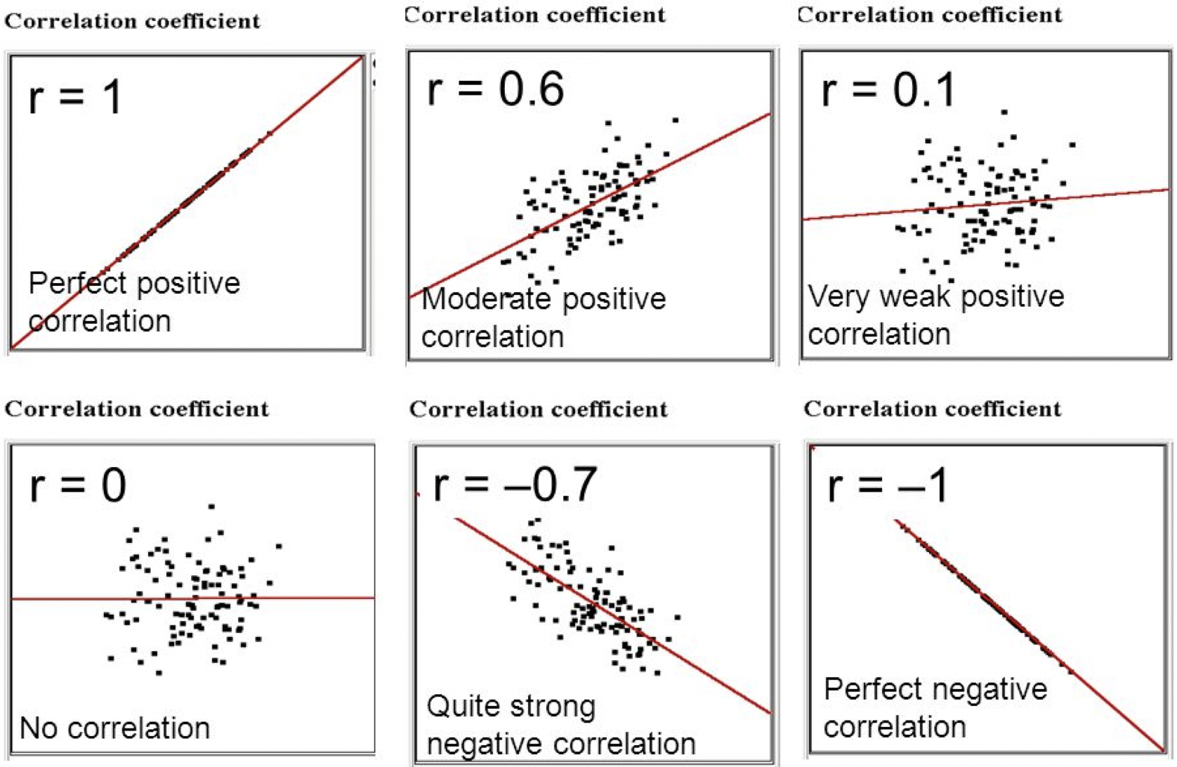
Correlation. We are interested in:
- Direction
  - Positive or negative
  - Slope of the line
- Strength (Weak/Moderate/Strong)
  - How close are the data points to the line
    - Very close = strong
    - Very dispersed = weak
    - Values closer to +1 or -1 indicate stronger relationship
- Statistical Significance
  - Likelihood the relationship we observe is occurring due to chance
Scatterplots. When to use:
- Bivariate numerical data (two variables)
- Plot the relationship between two variables
  - One independent (X - horizontal scale), one dependent (Y - vertical scale)
- Collection of ordered pairs
- Linear trend:
- Also can be curved
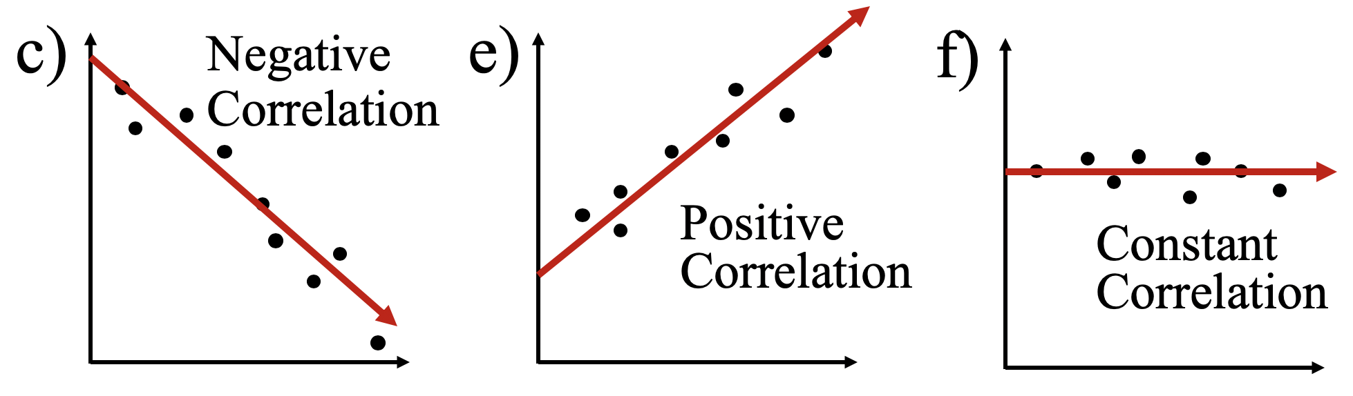
Positive Correlation:
- Both Y and X cordinates increase
- This means they are related
- eg.: age and height. As the child gets older, the child gets taller.
Negative Correlation:
- One of the cordinates (Y or X) increases while the other one decreases.
- It does make a downhill graph.
- This means the two are related as opposites.
- eg.: age of a car and its value. As the car gets older, the car is worth less.
Constant Correlation:
- ** One of the cordinates doesn’t change.
No Correlation
- If there seems to be no pattern, and the points looked scattered, then it is no correlation.
- Eg.: If you look at hair colour of boots a premier league footballer wears and their scoring average, you will find that there is no correlation between the two.
Eg.: children’s maths scores at age 16 and their achievement of a standard maths test at aged 7. We are interested to see if the score a child achieves at age 7 is related to the score they achieve at age 16.
y = b0 + bx + e
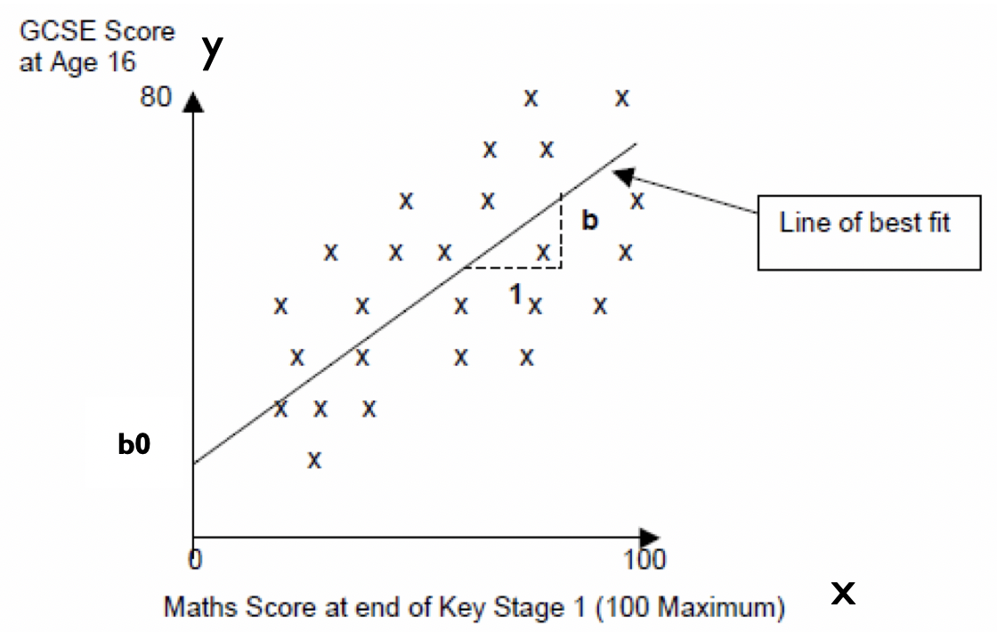
- b0 is the intercept or the point where the line crosses the y-axis (y value when x=0).
  - b0 is the gradient of the line
  - Represents the amount that the outcome variable changes for one unit change in the independent variable. e.g. for every one percentage point increase in a child’s Maths Test score, the line suggests that the child’s GCSE Score increases by ‘b’ points.
- e is basically the vertical distance between each point and the line itself.
  - Model is a best fit. e obviously varies. Without any further information about confounding variables we cannot explain this variation – so we include it as an error.
y = b0 + bx
- if we are dealing with a normal distribution these error terms will cancel each other out and we do not need to include it in the equation.
Eg of looking at Co-variation:
- Nutrition and growth
- Pollen and bees
- Violence on TV and violence in Society?
- Parametric
  - Make assumptions about the population from which the sample is taken
  - Shape of the population (normally distributed)
  - Eg.: Pearson’s Correlation
  - Normality: Scores should be normally distributed
    - Inspect histograms for each variable
  - Linearity: There must be a linear relationship between the two variables
    - Inspect a scatterplot and you should see a straight line not a curve
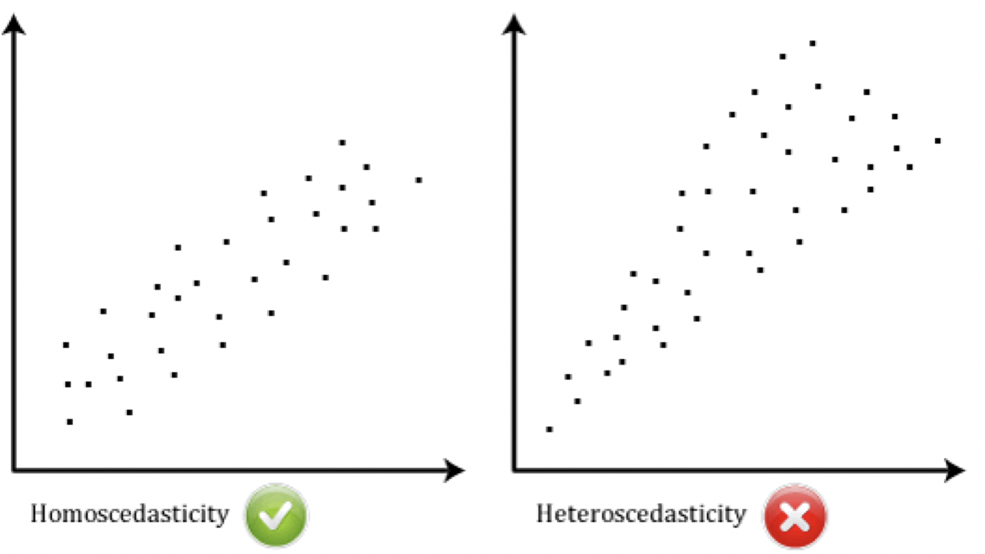
  - Homoscedasticity: Variability of variable 1 should be similar to variable 2
    - Check scatterplot. Looking at distance between the points to that straight line. The shape of the scatterplot should be tube-like or rectangular in shape. If the shape is cone-like, then homoscedasticity would not be met.
    - It is a matter of degree
    - heteroscedasticity: When doesn’t make sense to base any prediction in an homoscedasticity relationship. Eg.: income levels and spending on gadgets:
      - Strong relationship with income and spending.
      - But pattern graphically shows levels of spend low for low incomes and varies for those with high incomes. Therefore have heteroscedasticity which means that it doesn’t make sense to base any prediction based on this relationship
- Non-parametric
  - Do not make assumptions about the population and its distribution
  - Tolerant set of tests which don’t expect your data to anything fancy
    - Not high-powered and don’t promise more than they can deliver
    - May fail to detect differences that exist
  - Use for nominal or ordinal data
  - Use for small samples
  - Use for skewed data
  - Eg.: Spearman Rank Order Correlation
Measuring Relationships
- We assess the relationship via the correlation coefficient and by calculating the Covariance.
  - We look at how much each score deviates from the mean.
  - If both variables deviate from the mean by the same amount, they are likely to be related.
- We can look at a bi-variate correlation or a partial correlation
- Bi-variate: two variables
- Partial: two variables while controlling for another
Modeling Relationships
- First, look at some scatterplots of the variables that have been measured:
  - Outcome_i = (model) + error
  - Outcome_i = (bX_i ) + error
- Strength of relationships
Detrended Q-Q Plot
- The horizontal line at the origin represents the quantiles that we would expect to see if the data were normal;
- The dots represent the magnitude and direction of deviation in the observed quantiles.
- Each dot is calculated by subtracting the expected quantile from the observed quantile. (This implies that if a dot is below the trend line on the Normal Q-Q plot, it will appear above the trend line on the Detrended Normal Q-Q plot, because observed - expected > 0.)
Inspect a Scale Variable:
- Generate summary statistics
- Make sure you include skewness and kurtosis
- Generate a histogram with a normal curve showing
- Generate a Q-Q plot
- Review your statistics and plots to see how far away from normal your data is
Tests of Normality
- Estimates vary significantly from zero?
- Look at the standard error of skewness and kurtosis.
- Is the value of ‘zero’ is within the 95% Confidence Interval (CI)?
- Standardised scores (value/std.error) for skewness between -2 and +2 are considered acceptable in order to prove normal univariate distribution.
- Tpcois:
  - Standardised Skew = -.401/.118=-3.40 Standardised Kurtosis=.257/.236=1.08
- Skewnees is not acceptable
  - Look at the outliers, how many of them there are or whether we can transform it to become more normal.
So our data has failed the standardised skew. Does this mean we can’t use parametric tests?
- No! Do some additional checks: (see PSIWeek3-Lecture.Rmd)
  1. create a histogram to see how much skew there is.
  2. Convert the raw score for tpcoiss to a standardised score.
    - If 95% of our data falls within +/- 1.96 then we can treat the data as normal.
  3. sort it,. In R: scale(survey$tpcoiss)
    - will sort a list in ascending order.
  4. Check your Q-Q Plot
  5. Check skewness and kurtosis standardised scores
  6. Check impact of outliers
    - At 0.05 level if 95% of your data is within +/- 1.96 when converted to standardised scores – it is likely your data is safe to treat as normal
    - If the sample size is small (80 or fewer cases), a case is an outlier if its standard score is ±2.5 or beyond.
    - If the sample size is larger than 80 cases, a case is an outlier if its standard score is ±3.29 or beyond
  7. Pearson Correlation: Look at the distribution of both variables
    - Create a scatterplot
    - Look at outliers
    - Look at distribution of the data points
    - Run the correlation
    - Interpret the output
    - Check the information you have been given about the sample
    - Determine the direction of the relationship
    - Determine the strength of the relationship
    - Calculate the coefficient of determination
    - Assess the significance level
Correlation Analysis
Things to know about the Correlation Co-efficient (Key slide)
- It varies between -1 and +1
  - 0 = no relationship
- It is an effect size (ignore sign for magnitude of effect)
  - ±.1 = small/weak
  - ±.3 = medium/moderate
  - ±.5 = large/strong
  - Cohen’s effect size heuristic is standard
    - Find a book that is respected in your field that discusses this and cite it when stating you used Cohen’s convention
  - Coefficient of determination, r2
    - By squaring the value of r you get the proportion of variance in one variable shared by the other.
  - Significance of all co-efficient and covariance depends on the p-value (significance value of the test)
Reporting a Pearson correlation in words:
- “The relationship between Total PCOISS (derived from the PCOISS questionnaire) and Total Perceived Stress (derived from the perceived stress questionnaire) was investigated using a Pearson correlation. A strong negative correlation was found (r =-.580, n=424, p<.001).”
 
 NOTE1: Because the significance is .000 in test results, the convention is to report it as <.001 NOTE2: N=424 because it does not include missing values
Covariance
- Variance tells us by how much scores deviate from the mean for a single variable.
- Covariance = Scaled version of variance.
- The covariance is the average cross-product deviations:
  1. Calculate the error between the mean and each observations score for the first variable (x).
  2. Calculate the error between the mean and their score for the second variable (y).
  3. Multiply these error values. Add these values and you get the cross product deviations.
- It depends upon the units of measurement.
  - E.g. The Covariance of two variables measured in Miles might be 4.25, but if the same scores are converted to Km, the Covariance is 11.
- One solution: standardise it!
  - The standardised version of Covariance is known as the Correlation coefficient.
    - Divide by the standard deviations of both variables.
    - Create standardised scores
Hypothesis Testing
- Hypothesis may concern an effect (e.g. correlation) in the population or a difference between groups in a population.
- The general goal of a hypothesis test is to rule out chance (sampling error) as a plausible explanation for the results from a research study.
- All hypothesis testing starts with the null hypothesis : that there is no effect or difference in the population.
Hypothesis statement
- The null hypothesis, denoted by H₀, is a claim about a population characteristic that is initially assumed to be true.
- The alternative hypothesis, denoted by H_a, is the competing claim.
  - You are usually trying to determine if this claim is believable.
- The hypothesis statements are ALWAYS about the population. NEVER about a sample!
The Form of Hypotheses
- H₀: population characteristic = hypothesized value
 - The null hypotesis ALWAYS includes the equal case
 - “hypothesized value” is a specific number determined by context of the problem
- H₁: population characteristic > hypothesized value
 - Uses the same “population characteristic” and “hypothesized value”
 - The > is determined by context of the problem
- H₂: population characteristic < hypothesized value
 - Both H₁ and H₂ are considered one-tailed tests, becouse it shows interst in one direction ( > and < )
- H₃: population characteristic ≠ hypothesized value
 - Considered two-tailed tests, becouse it shows interst in both directions (≠)
When you perform a hypothesis test you make a decision:
- reject H₀ or fail to reject H₀
- (Key slide) Each could possibly be a wrong decision; therefore, there are two types of errors:
  - Type I:
    - The error of rejecting H₀ when H₀ is true
    - The probability of a Type I error is denoted by α (Alpha).
      - α is called the significance level of the test.
  - Type II:
    - The error of failing to reject H₀ when H₀ is false
    - The probability of a Type II error is denoted by β (Beta).

	H₀ is true	H₀ is false
Reject H₀	`Type I error`	Correct
Fail to reject </br>Reject H₀	Correct	`Type II error`

P-value, α – statistical significance (Key slide)
- A probability measure of evidence about H₀.
- Put simply it is the probability, given the null hypothesis is true, that the results could have been obtained purely on the basis of chance alone.
- The probability (under presumption that H₀ true) the test statistic equals observed value or value even more extreme predicted by H_α
- The P-value allows us to answer the question:
  - Do our sample results allow us to reject H₀ in favour of H_α?
  - If that probability (p-value) is small, it suggests the observed result cannot be easily explained by chance.
Statistical Significance (Key slide)
- Working with random samples can never have 100% certainty that findings we derive from the sample will reflect real differences in the population as a whole.
- Convention is that (for your field of study) there is an accepted level of probability such that it is considered so small that the finding from your sample is unlikely to have occurred by chance or sampling error.
- Normally, that line is drawn at p=0.05 or p=0.01.
  - In other words, when a statistical test tells us that the finding has less than a 5% or 1% chance of occurring due to sampling error then we tend to conclude that we can be sufficiently confident that the finding is therefore likely to reflect a ‘real’ characteristic of the population as a whole.
- When this occurs, you can say that your finding is statistically significant.
Statistical Significance
- A range of statistical tests can be used
  - Each will tell you how likely it is that a finding you get from your sample would occur simply by chance if no such difference actually existed in the population as a whole ie. the probability that your finding is simply a fluke occurrence deriving from the random selection of your sample.
Hypothesis test
- Using the standard level accepted by your domain (e.g. p ≤0.05 or p ≤0.01)
- If the probability less than this value then you reject the null hypothesis and thus accept the alternative hypothesis and you can state that your findings are statistically significant.
- If the probability is greater this value then you conclude that there is no evidence to reject the null hypothesis and your findings are not statistically significant.
  - N.B This is different from concluding that you have evidence to accept the null hypothesis. In these cases, your findings are said to be not significant.
- Caveat: If we get a p-value of 0.051 should we accept the null hypothesis? Should we reject the null hypothesis if we get a p-value of 0.049?
  - Need to allow for some flexibility in interpretation.
Accepting and Rejecting Hypotheses (Key slide)
- A non-statistically significant test result does not mean that the null hypothesis is true
- A significant result does not mean that the null hypothesis is false
Correlation and Causality
- The third-variable problem:
  - Causality between two variables cannot be assumed because there may be other measured or unmeasured variables affecting the results.
Spearman (Non-parametric)
- Doesn’t require normality
- Requires independent observations
- Use when assumptions of Pearson are violated or when data is not scale
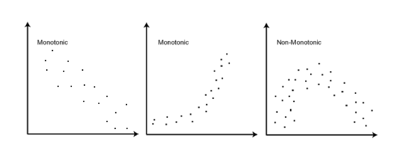
- Spearman - Requires a monontonic relationship – as one variable increases, so does the other or as one increases the other decreases

Spearman (Non-parametric)

Spearman’s Rho is the statistic in R (aka r_s or the Greek letter ρ) Kendall’s Tau is the statistic in R (aka tau-b or τ_b)

Tests for Group Comparison

	Independent Samples	Related Samples
Interval measures/ parametric	Independent samples t-test*	Paired samples t-test**
Ordinal/ non-parametric	Mann-Whitney U-Test	Wilcoxon test

* 2 different groups of participants ** 2 same participants measured at two different points

Parametric: t-tests
- Compare the mean between 2 samples/groups/conditions
  - If 2 samples are taken from the same population, then they should have fairly similar means
  - if 2 means are statistically different, then the samples are likely to be drawn from 2 different populations, i.e. they really are different
t Distribution
- Similar to the Z distribution by assuming normality.
- Normality is obtained after about 120 data observations.
 - In which case t = z
- Basic rule of parameter estimation:
 - The higher the observations (N) of sample the more reflective of overall population.
- The t distribution is a short, fat relative of the normal.
- The shape of t depends on its degrees of freedom.
- As N becomes infinitely large, t becomes normal and becomes z
- Only need to check if your sample is smaller than 120
 - See table
- Test statistic:
 - Difference between the means divided by the pooled standard error of the mean
 - t=(X̅₁–X̅₂)/(S_{X̅₁–X̅₂})
 
 Reporting convention: t= 11.456, df= 9, p< 0.001 (Remember df depends on the number in your sample)
- Both the independent t-test and the dependent t-test are parametric tests based on the normal distribution.
 - Data are measured at least at the interval level.
 - The sampling distribution is normally distributed.
 - In the dependent t-test this means that the sampling distribution of the differences between scores should be normal, not the scores themselves.
- Eg.:
 - Dataset created from a designed to explore the factors that impact on respondents’ psychological adjustment and wellbeing.
 - Question: Is there a significant difference in the mean self-esteem scores for males and females?
 - Need: One categorical variable (male/female gender) One continuous, dependent variable (self-esteem score tslfest)
 - T-test: Will tell you whether there is a statistically significant difference between the mean scores of the groups
 - We need to know the homogeneity of variance in advance so we can set the parameter on the t-test so we conduct the Levene’s test
 - Levene’s test is the most robust test for normally distributed data
 - (Fligner-Killeen test is a non-parametric test equivalent.)
Mann-Whitney test
- It is used to test the null hypothesis that two samples come from the same population (i.e. have the same median) or, alternatively, whether observations in one sample tend to be larger than observations in the other.
- Compares the medians from two populations and works when the Y variable is continuous and the X variable is discrete with two attributes.
  - Of course, the Mann-Whitney test can also be used for normally distributed data, but in that case it is less powerful than the 2-sample t-test.
Effect Size:
- convert a z-score into the effect size:
  - r=Z/√N̅

Lecture 4 - 10/10/2018

Difference

Sources of the class:
- Statistics and Data Analysis, Peck, Olsen and Devore;
- Discovering Statistics Using R, Field and Miles
- Understanding Basic Statistics, Brase and Brase
- SPSS Survival Manual, Julie Pallant
Webcourses portal: Download content (Week 4):

File experim.dat (3.964 KB)
File Field-BDI-Non-parametric.dat (466 B)
File L4 - Difference.pptx (1.66 MB)
File PSIWeek4-Lecture.html (790.572 KB)
File PSIWeek4-Lecture.Rmd (3.924 KB)
File Regression.sav (190.636 KB)
File survey.dat (192.817 KB)
File PSIWeek4Exercise.docx (198.268 KB)

Attached to this page you will find:

Lecture notes for this week
Rmd file plus Html output for rmd used in the lecture
Exercise for this week
Datasets used (regression.sav, survey.dat, Field-BDI-Non-Parametric.dat, experim.dat)

(Review class)

Lecture 5 - 17/10/2018

Comparing More Than Two Groups. Comparing non-numerical variables

Source of the class:
- Statistics and Data Analysis, Peck, Olsen and Devore;
- Discovering Statistics Using IBM SPSS, Andy Field;
- Understanding Basic Statistics, Brase and Brase;
- SPSS Survival Manual, Julie Pallant

File bullying.dat (69.664 KB)
File diet.dat (573 B)
File experim.dat (3.964 KB)
File L5 - Differences More than Two.pptx (1.88 MB)
File PSI-Lecture5.html (738.271 KB)
File PSI-Lecture5.Rmd (6.816 KB)
File survey.dat (192.817 KB)
File youthcohort.dat (3.185 MB)
This week we will be using the following R packages:

library(psych)library(semTools)library(stats)library(ggplot2)library(FSA)library(userfriendlyscience) library(gmodels)

Attached to this page are :

Lecture Notes for this week
Markdown file plus html output for R used in the lecture
Datasets used.

Comparison of more than 2 samples:
- ANOVA (ANalysis Of VAriance)

	Independent Samples	Related Samples
Interval measures/ parametric	ANOVA*	Repeated** Measures ANOVA
Ordinal/ non-parametric	Kruskall-Wallis	Freidman

* multiple different groups of participants ** multiple same participants measured at multiple different points

Still compares the differences in means between groups but it uses the variance of data to “decide” if means are different
- Really is ANOVASMD (Analysis of variance to see if means are different)
If the observed differences (btw variances of the groups) are a lot bigger than what you’d expect by chance, you have statistical significance.
Factors: the overall ‘things’ being compared (e.g. age, task, score)
Levels: the elements of the factor (young v old and naming v reading aloud)
F- statistic or F-ratio
- Magnitude of the difference between the different conditions
  - Similar to z or t-score as it compares the amount of systematic variance in the data to the amount of unsystematic variance.
- It is the ratio of the experimental effect to the individual differences in performance.
- Less than 1, it must represent a non-significant event (so you always want a F-ratio greater than 1)
- Degrees of freedom – depends on the number of factors and the number of levels
ANOVA tests for one overall effect only
- Omnibus test
There is a need for post-hoc testing
- ANOVA can tell you if there is an effect but not where
To test for significance
- obtained F-ratio is compared against maximum value one would expect to get by chance alone in an F-distribution with the same degrees of freedom.
- p-value associated with F is probability that differences between groups could occur by chance if null-hypothesis is correct
 
 Reporting convention: F= 65.58, df= 4,45, p< .001
F Distribution
- curve is skewed to the right.
- There is a different curve for each set of degrees of freedom (dfs)
- F statistic is greater than or equal to zero.
- As the degrees of freedom for the numerator and for the denominator get larger, the curve approximates the normal.
What Does ANOVA Tell us?
- Null Hypothesis:
  - Like a t-test, ANOVA tests the null hypothesis that the means of the different groups are the same.
- Alternate Hypothesis:
  - The means differ.
- ANOVA is an Omnibus test
  - It tests for an overall difference between groups.
  - It tells us that the group means are different.
  - It doesn’t tell us exactly which means differ.
Eg: One-way Between-Groups ANOVA

see PSI-Lecture5.Rmd
- Question: Is there a difference in optimism scores for young, middle-aged and old participants?
- Need: One independent variable with three or more levels (age category) (agegp3) One continuous variable (optimism scores) (totopt) Non-parametric equivalent: Kruskal-Wallis Test
One-way ANOVA will tell us whether there are significant differences in optimism scores (toptim) across the three groups (agegp3)
- Tell us if there is a difference but not where the difference is
 - need to conduct post-hoc tests after ANOVA to find it
 - Homocedascticity – Tukey’s honestly significant difference (HSD) post hoc test (Eg.: TukeyHSD(…))
 - Otherwise use Games-Howell
 - In R need to specify in relevant post-hoc test function
- Eg in IR:
```
 one.way <- oneway(sdata$agegp3, y = sdata$toptim, posthoc = 'Tukey')
```
Calculating the effect size
- eta squared = sum of squares between groups/total sum of squares (from our ANOVA output (rounded up))
- Guidelines on effect size: 0.01=small, 0.06=moderate, 0.14=large
Reporting results eg:
- A one-way between-groups analysis of variance was conducted to explore the impact of age on levels of optimism, as measured by the Life orientation Test (LOT). Participants were divided into three groups according to their age (Group 1: 29 yrs or less; Group 2: 30 to 44 yrs; Group 3: 45yrs and above). There was a statistically significant difference at the p < .05 level in LOT scores for the three age groups: F(2, 432)=4.6, p=.01. Despite reaching statistical significance, the actual difference in mean scores between groups was quite small. The effect size, calculated using eta squared was .02. Post-hoc comparisons using the Tukey HSD test indicated that the mean score for Group 1 (M=21.36, SD=4.55) was statistically different to Group 3 (M=22.96, SD=4.49). Group 2 (M=22.10, SD=4.15) did not differ significantly from either Group 1 or 3.
Bonferroni Correction
- corrects/adjusts the p value by dividing the original α-value by the number of analyses on the dependent variable.
  - needed as conducting multiple analyses between groups on the same dependent variable can inflate the chance of a Type I error: Incorrectly rejecting the null hypothesis
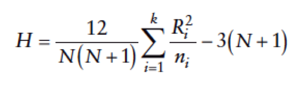
Kruskal–Wallis test – Non Parametric
- non-parametric counterpart of the one-way independent ANOVA (analysis of variance).
- It is based on ranked data.
- The sum of ranks for each group is denoted by Ri (where i is used to denote the particular group).
- Eg.: Question: Are there any differences between pupils of different ethnicity in England and Wales in relation to the grades they achieved in GCSE Maths?
- See youthcohort.dat analysis at PSI-Lecture5.Rmd
  - H0: There is no difference
  - HA: There is a difference
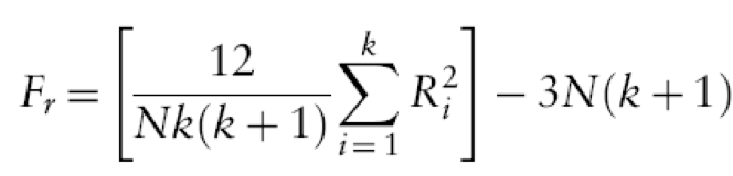
Friedman’s ANOVA
- Non-parametric test for differences between several related groups
- Used for testing differences between conditions when:
  - There are more than two conditions
  - The same participants have been used in all conditions (each case contributes several scores to the data).
- If you have violated some assumption of parametric tests then this test can be a useful way around the problem.
- it is based on ranked data.
- Once the sum of ranks has been calculated for each group, the test statistic, Fr, is calculated as:
- Eg.: Does the ‘andikins’ diet work?
  - See diet.dat analysis at PSI-Lecture5.Rmd
Comparing Nominal Values
- When two variables are independent, there is no relationship between them.
- See bullying.dat analysis at PSI-Lecture5.Rmd
- Question: Is there a difference between boys and girls in terms of whether they have been bullied at school?
  - H0: There is no difference
  - HA: There is a difference
Chi-square Test
- We are comparing observed values to expected values according to a specific hypothesis (null hypothesis)
- The null hypothesis for this test states that the proportions (the distribution across categories) are the same for all of the populations
- Views the data as two (or more) separate samples representing the different populations being compared
  - The same variable is measured for each sample by classifying individual subjects into categories of the variable.
  - The data are presented in a matrix with the different samples defining the rows and the categories of the variable defining the columns.
  - The data, called observed frequencies, simply show how many individuals from the sample are in each cell of the matrix.
- A chi-square statistic is computed to measure the amount of discrepancy between the ideal sample (expected frequencies from H0) and the actual sample data (the observed frequencies).
- Output is a cross tabulation table
  - See bullying.dat analysis at PSI-Lecture5.Rmd
Yate’s Continuity Correction
- Also to prevent use making a Type I error
- When we are doing a Chi-square test we are assuming that the probability distribution of the binomial frequencies observed approximate the Chi-square distribution
  - This is not quite correct. Yate’s correction adjusts Pearson’s Chi-square by subtracting 0.5 from each of the differences between the observed values and the expected values, which will reduce the Chi-square statistic and its associated p-value
  - Particularly important for small data (larger datasets this can be overcome)
  - May tend to overcorrect – make sure you reflect your research area’s perspective (some would say Yates is unnecessary even for small data).
Chi Square Statistic
- Measures the amount of discrepancy between the ideal sample (expected frequencies from H₀) and the actual sample data (the observed frequencies = f_o).
- A large discrepancy results in a large value for chi-square which indicates that the data do not fit the null hypothesis and the hypothesis does not hold.
- For one degree of freedom
  - The critical value associated with p=0.05 for Chi Square is 3.84
  - The critical value associated with p=0.01 it is 6.64
  - Chi-square values higher than this critical value are associated with a statistically low probability that H₀ holds.
Chi-Square Test for Independence (Reporting example)
- A Chi-Square test for independence (with Yates’ Continuity Correction) indicated no significant association between gender and reported experience of bullying, χ2(1,n=801)=2.30,p=.13, phi=-.056).
Repeated Measures Categorical Variables
- Use McNemar’s test
- Matched Samples or repeated measures (pre-test/post-test)
  - Two variables one recorded at Time 1 and one recorded at Time 2 (after an intervention)
- Use for categorical variables with two response options
  - For 3 or more use Cochran’s Q-test
Back to Hypothesis Testing
- Power of a Hypothesis Test
  - power β of a hypothesis test: the probability that the test will reject the null hypothesis when there is no effect.
  - The power of a test depends on a variety of factors including the size of the effect and the size of the sample.
- Power analysis
  1. sample size
  2. effect size
  3. significance level
    - P(Type I error) = probability of finding an effect that is not there
  4. power: P(Type II error) = probability of finding an effect that is there
    - Given any three, we can determine the fourth.

Lecture 6 - 24/10/2018

Assignment class revision. Descriptive statistics, graphs, tests

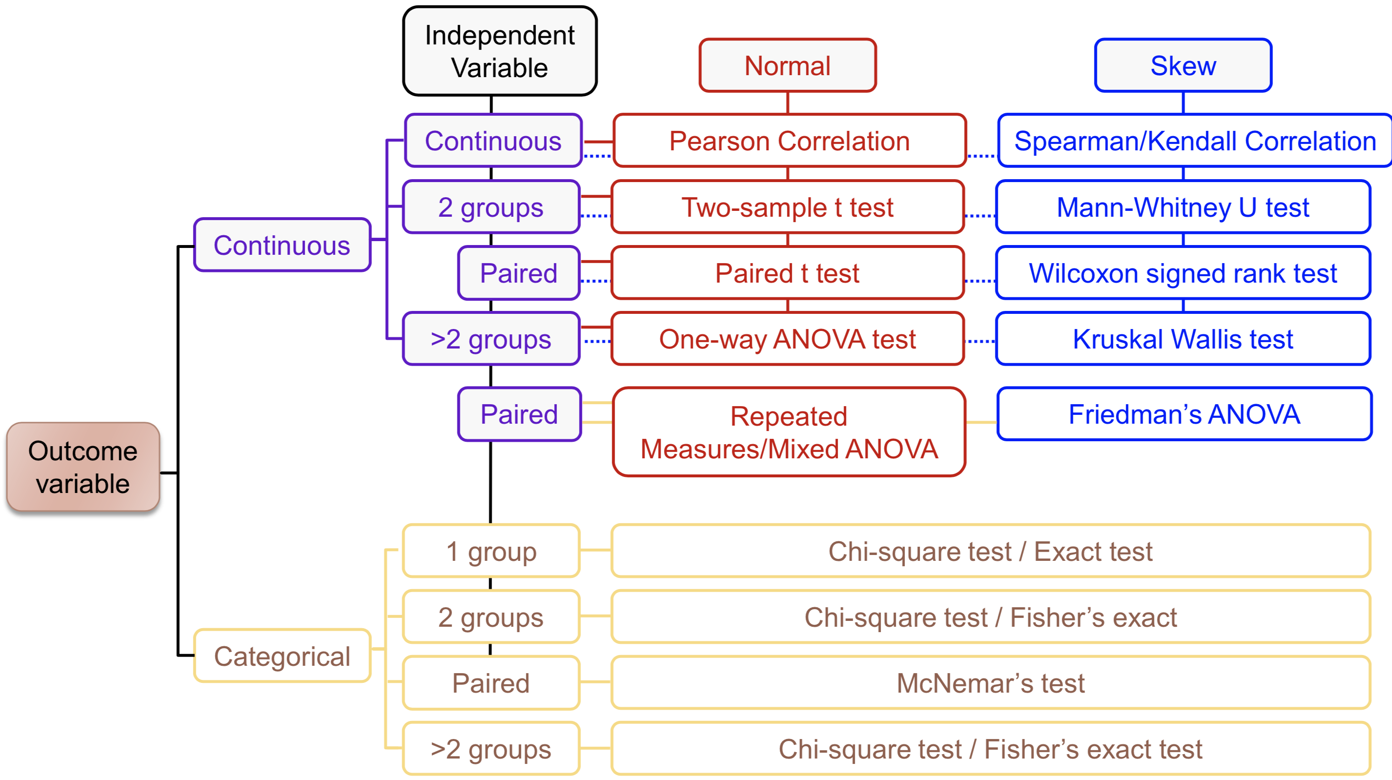
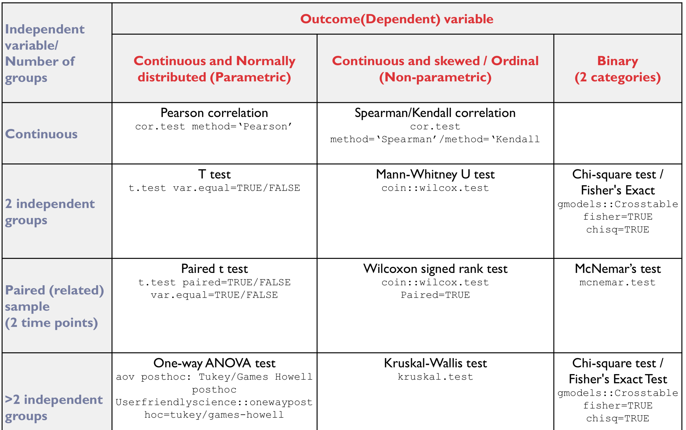
Module Link/Module Content/Choosing your Statistical Test (pdf)”

How to choose?
Parametric Difference Tests – Pre-Check
- T-test:
  - Levene’s test
    - Non-significant result variances homogenous in groups (var.equal=TRUE)
    - Significant result variances heterogeneous (var.equal=FALSE)
- ANOVA:
  - Bartlett’s test
    - Non-significant result variances homogeneous in groups (Tukey post-hoc)
    - Significant result variances heterogeneous (Games Howell post-hoc)
Outcome (Dependent) Variable

Lecture 6 - 07/11/2018 (week 8)

Dimension Reduction Linear Regression

Source of the class:
- Field, Miles and Field Discovering Statistics Discovering Statistics with R

File L6 - Dimension Reduction.pptx (8.889 MB)
File PSI-Lecture6-DimRed.html (1.934 MB)
File PSI-Lecture6-DimRed.Rmd (4.64 KB)
Attached to this page you will find:
---
File PSI-Lecture7-LinReg.html (725.91 KB)
File L7 - Getting Started with Predictive Statistics.pptx (1.914 MB)
File PSI-Lecture7-LinReg.Rmd (1.322 KB)
Attached to this page are:

Principal Component Analysis (PCA) and Factor Analysis
- Used to explore the relationship between one outcome variable and a set of independent variables (predictors)
- Inferential Model
  - Prediction: Really what we are looking at is the variance in the outcome variable and how much of the variance could be considered to be explained by the predictor variables
    - How well a set of variables is able to predict an outcome variable
    - Which variable in a set is the best predictor
    - Whether a variable is still able to predict an outcome when controlling for other variables
  - y=b₀+b₁x₁+b₂+b₂x₂…+b_nx_n+…ε_i
    - b0 is the intercept
      - the value of the Y variable when all Xs = 0.
      - point at which the regression plane crosses the Y-axis (vertical).
    - b1 to bn are the regression coefficient for variable 1 to n
  - Pseudo Prediction – if we use a linear equation
    - You must have a sound theoretical basis for including your variables
    - Explore the data using univariate and bivariate analysis to establish statistical evidence
    - Only include variables that have potentially informative results or which serve as controls
  - understand not only how your variables relate to your outcome but also to each other.
- Dimension reduction
  - **strives to avoid: **Using a single score/measure from a multi-item measure in which there is great heterogeneity; or
  - Using several scores/measures that are highly correlated or unreliable.
  - The goal is to obtain the “right” number of scores (and it might be one).
- Collinearity
  - Occurs when two or more independent variables contain strongly redundant information
  - If variables are collinear they are essentially measuring the same thing
  - There is not enough distinct information in these variables for inferential statistics to operate
  - If we conduct inferential statistics with collinear variables then the model will produce unreliable results
  - Need to check for collinearity by examining a correlation matrix that compares your independent variables with each other.
  - A correlation coefficient above 0.8 suggests collinearity might be present
  - Problems:
    - You are introducing bias
    - Over-representing a concept
    - Increasing possibility of a Type I error (rejecting H₀ when H₀ is true)
  - How to avoid:
    - Delete all but one of the collinear variables from the model
    - Combine them into an index mathematically (e.g. multiplying, adding etc.)
    - Estimate a latent variable using an appropriate data reduction technique
      - Factor analysis (FA)/Principal Component Analysis (PCA)
Dimension reduction / Factor Analysis
- Want to avoid two major obstacles:
  - Using a single variable created from a multi-item measure in which there is great heterogeneity; or
  - Using several variables that are highly correlated or unreliable.
- The goal is to obtain the “right” number of variables to represent a concept
- The basic issue is the degree of correlation among a set of items.
- We want to test for clusters of variables or measures.
- Or to see whether different measures are tapping aspects of a common dimension.
- We expect to find “clumps” of items sometimes, and these are called factors or components.
- Many phenomena cannot be measured directly – no measurement scale exists
- To work with these latent variables we must use manifest variables and construct a measurement scale from these
- We are theorizing that there is a single individual concept, or a small number of concepts, which lead to different manifestations
- We are trying to distil the underlying concept(s) from its manifestations
Applicability
- We may be interested in creating an agreed measure that will allow us to track changes over time
- We may be interested in exploring particular dimensions of a concept
- We may, pragmatically, be interested in reducing the number of variables we need to work with in an analysis
Factor Analysis
- Exploratory: Used in early stages of research to gather information about interrelationships between variables
- Confirmatory: Used later in research to confirm hypotheses about the structure underlying a set of variables
Principal Components Analysis
- Used when working with a set of uncorrelated variables which it has been well established that they measure the same underlying component (s)

Academic Corner

Here you find all my academic life shareable notes.